Markov Decision Process
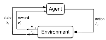
Let's start by defining the Markov Decision Process (MDP). Suppose we have a set of states $S$, a set of actions $A$, a transition function $P(s'|s, a)$, a reward function $R(s, a, s')$, a discount factor $\gamma$, a start state $s_0$, and the number of steps (i.e., Horizon) $H$.

The MDP is illustrated in the above diagram, where the agent starts at state $s_0$, and takes action $a$ at state $s$, then the environment transitions to state $s'$ with probability $P(s'|s, a)$, and the agent receives reward $R(s, a, s')$. The goal is to find the optimal policy $\pi$ that maximizes the expected reward: $$V^*(s) = \max_{\pi} \mathbb{E} \left[ \sum_{t=0}^{H} \gamma^t R(s_t, a_t, s_{t+1}) \mid s_0 = s \right]$$ where $V^*(s)$ is the optimal value function (i.e., sum of discounted rewards when starting from state $s$ to the end of the horizon $H$ under the optimal policy $\pi^*$).

Value Iteration
Let's start by thinking about how to compute the optimal value recursively :

• $V_0^*(s)$ denotes the optimal value for state $s$ when the horizon $H = 0$. Since the horizon is 0, there's no action to take, and we will just assume the value of doing nothing is 0 in this case: $V_0^*(s) = 0 \quad \forall s$.
• $V_1^*(s)$ denotes the optimal value for state $s$ when the horizon $H = 1$. The agent can take one action, and we should choose the action that maximizes reward after taking that action (note that the transition is not deterministic so we need to consider all possible next states $s'$):
  $$V_1^*(s) = \max_{a} \sum_{s'} P(s'|s, a) \left[ R(s, a, s') + \gamma V_0^*(s') \right]$$
• Similarly, we can recursively define $V_2^*(s)$ as: $$V_2^*(s) = \max_{a} \sum_{s'} P(s'|s, a) \left[ R(s, a, s') + \gamma V_1^*(s') \right]$$
• In general, we can recursively define $V_k^*(s)$ as: $$V_k^*(s) = \max_{a} \sum_{s'} P(s'|s, a) \left[ R(s, a, s') + \gamma V_{k-1}^*(s') \right]$$ This is known as the Bellman equation for $V_k^*(s)$.

We can therefore write out the value iteration algorithm as follows:
where the optimal policy is simply greedy with respect to the value function. In this setting, value iteration is guaranteed to converge to the optimal value function $V^*(s)$. To see why, let us denote $V^*_H(s)$ as the optimal value for $H$ steps, and $V^*(s)$ as the optimal value for infinite steps. The additional reward collected over additional time steps $H+1, H+2, \ldots$ is: $$\gamma^{H+1} R(s_{H+1}) + \gamma^{H+2} R(s_{H+2}) + \ldots \leq \gamma^{H+1} R_{max} + \gamma^{H+2} R_{max} + \ldots = \frac{\gamma^{H+1}}{1-\gamma} R_{max}$$ Since $0 < \gamma < 1$, the additional reward goes to 0 as $H$ goes to infinity.

We can do Q-value iteration in a similar way. We define $Q^*(s, a)$ as the expected utility starting in state $s$, taking action $a$, and then following the optimal policy. We can write out the Bellman equation for $Q^*(s, a)$ as: $$Q^*(s, a) = \sum_{s'} P(s'|s, a) \left[ R(s, a, s') + \gamma \max_{a'} Q^*(s', a') \right]$$ We can easily plug this into the value iteration algorithm to get the Q-value iteration algorithm, where the update step does: $$Q_k^*(s, a) = \sum_{s'} P(s'|s, a) \left[ R(s, a, s') + \gamma \max_{a'} Q_{k-1}^*(s', a') \right]$$ And the optimal policy is greedy with respect to the Q-value function: $$\pi_k^*(s) = \arg \max_{a} Q_k^*(s, a)$$ Policy Iteration
For a given policy $\pi(s)$, if it's deterministic, we can evaluate the value function $V^\pi(s)$ as: $$V^\pi(s) = \sum_{s'} P(s'|s, \pi(s)) \left[ R(s, \pi(s), s') + \gamma V^\pi_{k-1}(s') \right]$$ And if the policy is stochastic where $\pi(a|s)$ is the probability of taking action $a$ in state $s$, we can evaluate the value function $V^\pi(s)$ as: $$V^\pi(s) = \sum_{a} \pi(a|s) \sum_{s'} P(s'|s, a) \left[ R(s, a, s') + \gamma V^\pi(s') \right]$$ Previously in value iteration and Q-value iteration, there's no explicit policy update step: we always adopt a greedy policy and only update the value (or Q-value) function. In the policy iteration algorithm, we alternate between policy evaluation and policy improvement steps: The crucial difference between policy iteration and value iteration is that policy iteration would fix the current policy first and update the value function until convergence, and then update the policy based on the fixed value function. On the other hand, value iteration just keeps doing the Bellman update until convergence.

Max-Entropy RL
Reminder entropy measures uncertainty and is computed as: $$H(p) = \sum_i p(x_i) \log \frac{1}{p(x_i)} = - \sum_i p(x_i) \log p(x_i)$$ While the regular formualtion of RL aims to find (ignoring the discount factor): $$\max_{\pi} \mathbb{E} \left[ \sum_{t=0}^{H} R_t \right]$$ The max entropy formulation aims to find: $$\max_{\pi} \mathbb{E} \left[ \sum_{t=0}^{H} ( R_t + \beta H(\pi(\cdot|s_t)) ) \right]$$ This helps us find a distribution of near-optimal policies rather than collapsing to one. To solve it, let's first quickly recap constrained optimization. Suppose we want to solve: $$\max_{x} f(x) \quad \text{subject to} \quad g(x) = 0$$ The Lagrangian is: $$\mathcal{L}(x, \lambda) = f(x) + \lambda g(x)$$ and the dual problem is: $$\min_{\lambda} \max_{x} \mathcal{L}(x, \lambda) = \min_{\lambda} \max_{x} f(x) + \lambda g(x)$$ At the optimal point, the gradient of the Lagrangian with respect to $x$ should be 0: $$\frac{\partial \mathcal{L(x, \lambda)}}{\partial x} = 0, \quad \frac{\partial \mathcal{L(x, \lambda)}}{\partial \lambda} = 0$$ If we plug this into an one-step max-ent RL objective, we get: $$\max_{\pi(a)} E[r(a)] + \beta H(\pi(\cdot|s)) = \max_{\pi(a)} \sum_{a} \pi(a) r(a) - \beta \sum_{a} \pi(a) \log \pi(a)$$ $$\min_{\lambda} \max_{\pi(a)} \mathcal{L(\pi(a), \lambda)} = \sum_{a} \pi(a) r(a) - \beta \sum_{a} \pi(a) \log \pi(a) + \lambda (\sum_{a} \pi(a) - 1)$$ Solve for $\pi(a)$ by setting the gradient to 0, we get: $$\pi(a) = \frac{1}{Z} \text{exp}(\frac{1}{\beta} r(a)), \quad Z = \sum_{a} \text{exp}(\frac{1}{\beta} r(a))$$ Plugging this back into the objective, we get the optimal value: $$V = \beta \log \sum_{a} \text{exp}(\frac{1}{\beta} r(a))$$ Now let's consider the multi-step case. Our objective is: $$\max_{\pi} \mathbb{E} \left[ \sum_{t=0}^{H} ( r_t + \beta H(\pi(\cdot|s_t)) ) \right]$$ As in value iteration, we can write out the Bellman equation for the value function: \begin{align*} V_k(s) &= \max_{\pi} \mathbb{E}\left[ \sum_{t = (H-k)}^{H} \left( r_t + \beta H(\pi(a_t \mid s_t)) \right) \right] \\ &= \max_{\pi} \mathbb{E}\left[ r(s, a) + \beta H(\pi(a \mid s)) + \gamma V_{k-1}(s') \right] \\ &= \max_{\pi} \mathbb{E}\left[ Q_k(s,a) + \beta H(\pi (a \mid s)) \right] \\ \end{align*} where $Q_k(s,a) = E [r(s, a) + V_{k-1}(s')]$. The above reduces to the one-step case with $Q$ instead of $r$. We can directly trasnscribe the solution: $$V_k(s) = \beta \log \sum_{a} \text{exp}(\frac{1}{\beta} Q_k(s,a))$$ $$\pi_k(a|s) = \frac{1}{Z_k} \text{exp}(\frac{1}{\beta} Q_k(s,a)), \quad Z_k = \sum_{a} \text{exp}(\frac{1}{\beta} Q_k(s,a))$$ You can recognize that this is taking the softmax of the Q-value function: $$\pi_k(a|s) = \text{softmax}(\frac{1}{\beta} Q_k(s,a))$$ where $\beta$ functions like a temperature parameter. When $\beta \to 0$, the policy becomes greedy. When $\beta \to \infty$, the policy becomes uniform.

Q Learning
In the tabular setting so far (finite number of states and actions), remember we defined Q-value as the expected return you’ll get if you start in state $s$ and take action $a$ now. You can get the optimal Q-value (i.e., following the optimal policy after taking action $a$) by using the Bellman equation: $$Q^*(s,a) = \sum_{s'} P(s'|s, a) \left[ R(s, a, s') + \gamma \max_{a'} Q^*(s', a') \right]$$ Based on this, we have the Q-value iteration algorithm: $$Q_{k+1}(s,a) \leftarrow E_{s' \sim P(s'|s, a)}[R(s, a, s') + \gamma \max_{a'} Q_k(s', a')]$$ Instead of enumerating all possible next states $s'$, we can use a sample-based approach to estimate the Q-value: Note that tabular Q-learning is model-free, i.e., we don't need to know the transition model $P(s'|s, a)$. This is the main difference between tabular Q-learning and Q-value iteration, and it allows us to learn the Q-value function from data in unknown or complex environments. When sampling actions, we usually use an $\epsilon$-greedy policy: choose a random action with probability $\epsilon$ and choose the greedy action with probability $1-\epsilon$.

This means that Q-learning is an off-policy algorithm, i.e., we are using the greedy action to update the Q-value function, but we are sampling actions from a different policy (the $\epsilon$-greedy policy). Nevertheless, it still converges to the optimal Q-value function as long as we satisfy the following two conditions:

• All states and actions are visited infinitely often.
• The learning rate $\alpha$ decays appropriately such that for each $(s,a)$ pair: $\sum_{t=0}^{\infty} \alpha_t(s,a) = \infty$ and $\sum_{t=0}^{\infty} \alpha_t^2(s,a) < \infty$.

Now let's think beyond the tabular setting. Enumerating all states is impossible for more complex environments, and so instead of learning a table of Q-values, we need a parameterized Q function $Q_\theta(s,a)$ (e.g., a neural network). We can still compute the target in a similar way: $$\text{target} = R(s,a,s') + \gamma \max_{a'} Q_{\theta_k}(s', a')$$ But the update rule is now to fit update the parameters of the neural network to fit the target: $$\theta_{k+1} \leftarrow \theta_k - \alpha \nabla_{\theta} [\frac{1}{2} (Q_{\theta_k}(s,a) - \text{target}(s'))^2]$$ Combining this with experience replay, we get the Deep Q-Learning algorithm from the DeepMind DQN paper:

References:

• Foundations of Deep RL by Pieter Abbeel
• Stanford CS234 by Emma Brunskill